How Does Faster R-CNN Work: Part I

Understanding Faster R-CNN from the Perspective of Implementation

Xander CAI

Last updated on Apr 1, 2021 10 min read Object Detection

source: awesomeopensource.com

In the field of object detection, Faster R-CNN has shown great vitality. Although it was published in 2015, it is still the basis of many object detection algorithms, which is very rare in the rapidly changing field of deep learning. Fast R-CNN is also applied to more fields, such as pose estimation, object tracking, instance segmentation and image description.

This article will try to explain the architecture of Faster R-CNN from the perspective of implementation. As Fast R-CNN has a complex process and many symbols, it is easy to be confused. Thus, here vgg16 is taken as an example, and all illustrations and variables are based on VGG-16 + VOC2007.

1 Object Detection

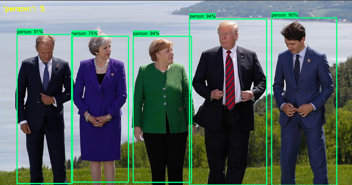
After the image classification issue was resolved by CNNs, the algorithm can tell what a picture is, but what if there are multiple objects in a picture, or people want to know where the objects are? Object detection algorithms are proposed. The below figure illustrates the difference between image classification, object detection and instance segmentation.

Figure 1: Comparison between image classification, object detection and instance segmentation (source: [1])

1.1 Dataset

In object detection field, COCO, Pascal VOC and ImageNet are well-known datasets, researchers publish results of their algorithms applied to them.

1.2 Metric

The commonly used metric used for object detection challenges is called the mean Average Precision (mAP). The mAP score is calculated by taking the mean AP over all classes and/or overall IoU thresholds, depending on different detection challenges that exist. Here is a detailed explanation.

1.3 R-CNN Family

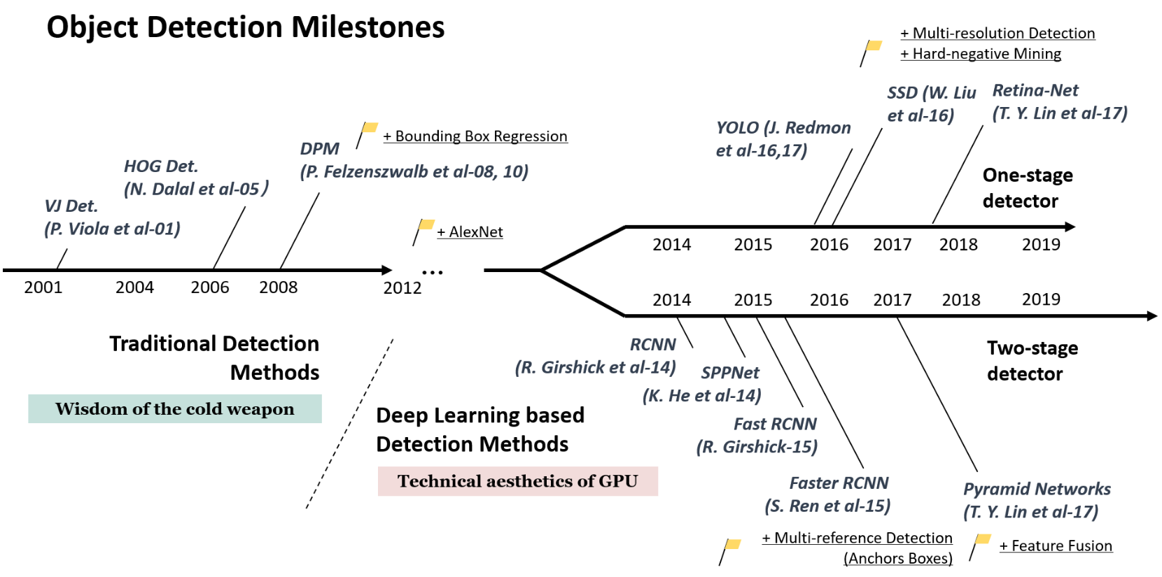
Figure 2: Object Detection Malestones (source: [2])

From the above milestones figure there are two methodologies to detect objects: one-stage detector and two-stage detector. Faster R-CNN inherited and developed former two-stage detectors: R-CNN, SPPNet and Fast R-CNN.

The three detectors in the R-CNN family:

R-CNN

Figure 3: R-CNN Architecture (source: [3])

The R-CNN detector first generates region proposals using an algorithm such as Edge Boxes. The proposal regions are cropped out of the image and resized. Then, the CNN classifies the cropped and resized regions. Finally, the region proposal bounding boxes are refined by a support vector machine (SVM) that is trained using CNN features. [3]

Fast R-CNN

Figure 4: Fast R-CNN Architecture (source: [3])

As in the R-CNN detector, the Fast R-CNN detector also uses an algorithm like Edge Boxes to generate region proposals. Unlike the R-CNN detector, which crops and resizes region proposals, the Fast R-CNN detector processes the entire image. Whereas an R-CNN detector must classify each region, Fast R-CNN pools CNN features corresponding to each region proposal. Fast R-CNN is more efficient than R-CNN, because in the Fast R-CNN detector, the computations for overlapping regions are shared. [3]

Faster R-CNN

Figure 5: Faster R-CNN Architecture (source: [3])

The Faster R-CNN detector adds a region proposal network (RPN) to generate region proposals directly in the network instead of using an external algorithm like Edge Boxes. The RPN uses Anchor Boxes for Object Detection. Generating region proposals in the network is faster and better tuned to your data. [3]

2 Faster R-CNN Architecture

The original paper [4] of the Faster R-CNN define the architechture as below figure:

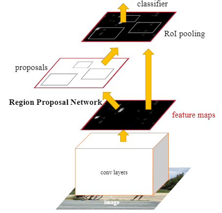
Figure 6: Diagram fo Faster R-CNN (source: [4])

Based on above figure, Faster R-CNN Can be divided into four main parts:

Conv Layers. A base network extract the feature map.
Region Proposal Networks (RPN). RPN generates anchors and output region proposals.
Region of Interest (RoI) Pooling. This layer maps the feature map in the proposal to target dimensions.
Classifier. It output the final classes and bounding boxs.

After understanding the Faster R-CNN architecture from the original paper, we can follow the above four main parts to implement it. The original implementation of Faster R-CNN was written in MATLAB, while the author, Ross Girshick, wrote a python version using Caffe [5], below figure shows the architecture of this detector based on pascal_voc/VGG16/faster_rcnn_alt_opt/faster_rcnn_test.pt file.

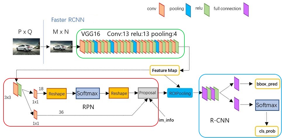
Figure 7: Faster R-CNN Architecture of faster_rcnn_test.pt

From the above figure, after finishing training the network, it processes an image of size P*Q with the following steps in the four main parts:

VGG16: resize the input P*Q image to fixed size M*N, and extract the feature map. The output feature map is fixed size (M/16)*(N/16)*512.
RPN: generate anchors, get probabilites of positive/negative anchors, calculate bounding box regression offset, and output proposals $[x_{1}, y_{1}, x_{2}, y_{2}]$.
RoI Pooling: collect proposals, generate fixed size proposal feature maps pooled_w*pooled_h.
R-CNN: classify proposal feature maps to get class probabilites and calculate bounding box regression of each proposal to get the final bounding box prediction.

3 Implementation

After sorting out the architecture and basic processing flow, we now look into the implementation of the four main parts.

3.1 Conv Layers

The Conv Layers is the base network of Faster R-CNN, the original paper chose ZFnet and VGG16 as the base network. There is no real consensus on which network architecture is best, other networks such as ResNet, Inception, DenseNet are common architectures for implementation. In this article, we only use VGG16.

Pre-processing

Each image need to be processed to fit base network. For VGG16, it need to be 0-255 bit BGR format, no bigger than 1000*600, and subtract an average value so that the average value of the image pixels is 0.

Base Network

Here the base network is the VGG16 without the full connection layers and output layer, and employs the pretrained model from Caffe. In the base network:

conv layer: kernel_size=3, pad=1, stride=1
pooling layer: kernel_size=2, pad=0, stride=2

In this way, the conv layers do not change the feature maps size, but the pooling layer will half the feature maps size. There are four pooling layers, thus, the output scale of the base network is 1/16.

3.2 Region Proposal Networks (RPN)

Faster R-CNN abandons the traditional sliding window and Selective Search (SS) method, and directly uses RPN to generate the detection frame, which is the advantage of Faster R-CNN that can greatly improve the generation speed of detection frames (2s -> 0.01s).

Anchors

We previously mentioned anchors several times, but what are anchors?

In the original paper, the author defines anchors as “reference boxes”. Anchors are fixed bounding boxes that are placed throughout the image with different sizes and ratios that are going to be used for reference when first predicting object locations. [6] If we run the generate_anchors.py [5] file, it generate below output:

[[ -84.  -40.   99.   55.]
 [-176.  -88.  191.  103.]
 [-360. -184.  375.  199.]
 [ -56.  -56.   71.   71.]
 [-120. -120.  135.  135.]
 [-248. -248.  263.  263.]
 [ -36.  -80.   51.   95.]
 [ -80. -168.   95.  183.]
 [-168. -344.  183.  359.]]

Each line represents the left top coordinate and right down coordinate of an anchor. By default we use 3 scales ($128^2$, $256^2$, $512^2$) and 3 aspect ratios (1:1, 1:2, 2:1), there are 9 (by default) anchors on each point of feature map, as shown at the left and right of the following figure, the location of each anchor centre is as shown at the centre in the above figure.

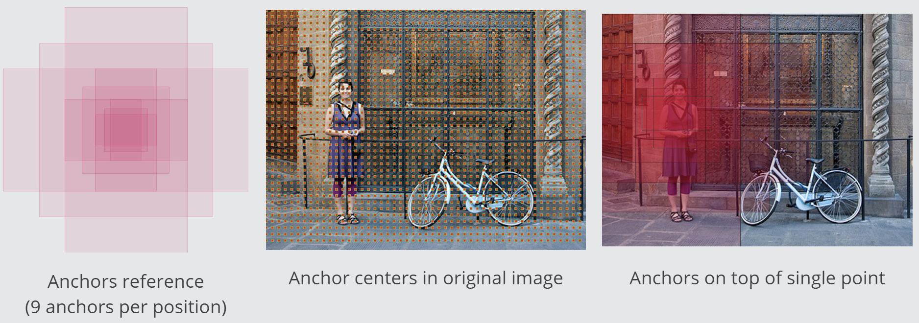
Figure 8: Anchors Representation (source:[6])

For VGG16, the anchor number of a M*N image is (M/16)*(N/16)*k (typically ~2,400), the anchors cover the images fully.

Proposal Layer

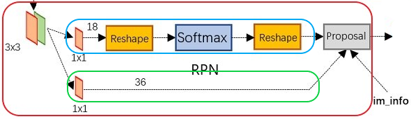
Figure 9: RPN data flow

The above figure shows the RPN structure, the input of RPN is a feature map from conv layer, there are two data flows, the upper flow classifies the anchors with positive or negative labels, the lower flow calculates the offset of bounding box regression. Then both flows combine in a Proposal layer to generate and filter suitable proposals.

In Faster R-CNN, a M*N image is transfored to a (M/16)*(N/16)*512 feature map. Let’s take M/16 as W, N/16 as H. From upper data flow (the blue frame in Figure 9), we see the W*H*512 featrue map is filtered by a 1*1*18 conv layer, the purpose is mapping 512 dimention feature map to 2*9 (positive/negative of 9 anchors) dimention vectors to classify positive or negative anchors. Then we send the WH18 feature map to softmax classifier to get positive or negative probility for each anchor.

In other words, RPN set up a dense number of candidate anchors on the scale of the original image, then use the base network to classify which anchors are positive (covering the ground truth) and which are negative anchors (outside the ground truth). Eventually, it turns out to solve a binary classification issue.

From lower data flow (the green frame in figure 9), we see the W*H*512 feature map is filtered by a 1*1*36 conv layer, the purpose is mapping 512 dimension feature map to 4*9 (four variables of 9 anchors) dimension vectors to run bounding box regression in the proposal layer. The four variables are centre coordinates of the anchor, and the width and height of the anchor are: $[d_{x}(A),d_{y}(A),d_{w}(A),d_{h}(A)]$.

Now the data flows send classification probabilites and regression vectors to the proposal layer, it processes those data by the following steps:

Generate anchors again, and run bounding box regression for all the anchors using $[d_{x}(A),d_{y}(A),d_{w}(A),d_{h}(A)]$.
Sort anchors based on the positive softmax score, keep the first NN (e.g. 6,000) number anchors.
Restrain the image boundary based on the positive anchors that beyond the image boundary, to prevent proposals crossing the image border in the RoI Pooling layer.
Remove small positive anchors.
Process the rest positive anchors using nonmaximum suppression (NMS) to remove duplicate proposals.
Output the final proposals (Regin of Interests, RoIs, i.e. the left top and right down of anchor coordinates), .

In brief, the key points of the RPN are:

generate anchors -> classify positive anchors -> bounding box regression for positive anchors -> generate proposals

3.3 Region of Interest (RoI) Pooling

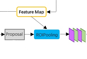
Figure 10: RoI Pooling Layer

As shown in the above figure, the RoI Pooling layer receives proposals from RPN and the feature map from the base network. The main task of the layer is extracting feature maps covered by proposals. Here is the problem: the proposals are not fixed-size boxes, but fixed-size feature maps are needed for the R-CNN in order to classify them into a fixed number of classes.

To solve this issue, Faster R-CNN uses RoI Pooling derived from Spatial Pyramid Pooling. The method is simple, assuming the proposal size is M*N, the fixed feature map size is pooled_w*pooled_h:

Get RoI: transfor proposal from the real image space to the feature map space, 1/16 scale.
Divide RoI: divide the feature map area that corresponds to the proposal into pooled_w*pooled_h grids, and perform round down if it cannot divide exactly.
Max pooling: Run max pooling for each grid.

Figure 11: RoI Pooling Operation (source:[7])

The above figure shows the RoI pooling operation of a 4*6 vector by a 3*3 conv core.

3.4 Region-based Convolutional Neural Network (R-CNN)

The R-CNN receives proposal feature maps from RoI pooling layer, and runs classification and bounding box regression again to get final classes probabilites and bounding box prediction, as shown in the following figure.

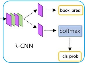
Figure 12: R-CNN Layer

In the original paper, the R-CNN takes the feature map for each proposal, flattens it and uses two fully-connected layers of size 4096 with ReLU activation. Then, it uses two different fully-connected layers for each of the different objects, assuming N is the total number of classes:

A fully-connected layer with N+1 units, the extra one is for the background class.
A fully-connected layer with 4N units of $[d_{x}(A),d_{y}(A),d_{w}(A),d_{h}(A)]$ for each of the N possible classes.

4 Summary

In this article, we illustrate the architecture of Faster R-CNN trying to understand how Faster R-CNN works, as the preparation for implementing it using PyTorch (Part II).

Generally, Faster R-CNN fully utilizes the base network, creates RPN to mark the target bounding box, employ RoI pooling to unify feature map in the bounding box, and gets final classes and bounding box in the R-CNN.

There are many details about NMS, bounding box regression, Intersection over Union (IoU), training RPN, training R-CNN etc., for the time limit, we have to leave it to Part II to illustrate them.