How Does Faster R-CNN Work: Part II

Last updated on Apr 20, 2021 19 min read

https://github.com/chenyuntc/simple-faster-rcnn-pytorch

This article will try to explain the architecture of Faster R-CNN from the perspective of implementation. Part II selected a simple method of implementation from github[1], the total code line number is under 2,000, and the performance is as good as the original paper.

1 Architecture

Based on Part I, The overall flow of Faster R-CNN is shown in the following figure.

Figure 1 Processing Flow Chart

The main components of the Faster R-CNN are Dataset, Extractor, RPN, RoIHead.

Dataset: provide data formats that meet the requirements.
Extractor: extract image features using CNN.
RPN: responsible for providing RoIs.
RoIHead: responsible for classification and fine tuning of RoIs.

The overall process of the Faster R-cnn can be divided into three steps:

Extracting: The image features are extracted from the pre-trained network.
Region Proposal: By using the extracted features, a certain number of RoIs are found through RPN network.
Classification and Regression: Input RoIs and image features into RoIHead to classify the RoIs, classify which categories, and fine tune the positions of RoIs.

The network architecture is shown in the following figure.

Figure 2 Network Achitecture

The project files are organized as following structre.

.
├── data
│   ├── __init__.py
│   ├── dataset.py
│   ├── util.py
│   └── voc_dataset.py
├── model
│   ├── __init__.py
│   ├── faster_rcnn.py
│   ├── faster_rcnn_vgg16.py
│   ├── region_proposal_network.py
│   └── utils
│       ├── __init__.py
│       ├── bbox_tools.py
│       └── creator_tool.py
├── trainer.py
├── train.py
└── utils
    ├── array_tool.py
    ├── config.py
    ├── eval_tool.py
    ├── __init__.py
    └── vis_tool.py

2 Implementation

2.1 Data Preprocessing

For each image, the following data processing is needed:

The image is scaled so that the long side is less than or equal to 1,000 and the short side is less than or equal to 600 (at least one is equal to).
The corresponding bounding boxes are also scaled at the same scale.
For VGG16 pre-training model of Caffe, the picture should be in 0-255, BGR format, and a mean value should be subtracted to make the mean value of the picture pixel 0.

Finally, four values are returned for model training:

images: BGR 3 channel image data plus width and height.
scale: zoom scale of original image $H\times W$ to preprocessed image $H'\times W'$, $scale = H/H'$.
bboxes: [Y_min, X_min, Y_max, X_max], bounding box coordinates of top left and down right.
labels: [label], [0-19] for VOC dataset.

2.2 Top Level

The three steps of Faster-RCNN:

Feature extraction: input a picture to get its feature map.
RPN: a series of RoIs are generated after a given feature map.
Positioning and classification: use the feature maps corresponding to these RoIs to classify the categories in these RoIs and improve the positioning accuracy

The top level of Faster R-CNN can be defined as below:

Class FasterRCNN

class FasterRCNN(nn.Module):
    def __init__(self, extractor, rpn, head):
        super(FasterRCNN, self).__init__()
        self.extractor = extractor
        self.rpn = rpn
        self.head = head

   def forward(self, imgs, scale=1.):
        img_size = imgs.shape[2:] # WxH
        features = self.extractor(imgs)
        rpn_locs, rpn_scores, rois, roi_indices, anchor = self.rpn(features, 
                                                                   img_size, 
                                                                   scale)
        roi_cls_locs, roi_scores = self.head(features,
                                             rois, 
                                             roi_indices)
        return roi_cls_locs, roi_scores, rois, roi_indices

These three important steps are initialized in the class FasterRCNN:

self.extractor
self.rpn
self.head

The function forward implements forward propagation is as shown in the following figure.

Figure 3 Forward Propagation

When choose VGG16 as backbone network, related parameters and settings can be defined.

Define Extractor, RPN, and Head as below:

Class FasterRCNNVGG16

class FasterRCNNVGG16(FasterRCNN):
    feat_stride = 16  # downsample 16x for output of conv5 in vgg16

    def __init__(self,
                 ratios=[0.5, 1, 2],
                 anchor_scales=[8, 16, 32]
                 ):
                 
        extractor, classifier = decomp_vgg16() # decomposition VGG16

        rpn = RegionProposalNetwork(
            512, 512, # channel number of input and internal feature map
            ratios=ratios,
            anchor_scales=anchor_scales,
            feat_stride=self.feat_stride,
        )

        head = VGG16RoIHead(
            n_class=n_fg_class + 1, # classes number plus background
            roi_size=7, # feature map size for roi pooling
            spatial_scale=(1. / self.feat_stride),
            classifier=classifier
        )

        super(FasterRCNNVGG16, self).__init__(
            extractor,
            rpn,
            head,
        )

2.3 Extractor

Extractor uses a pre-trained model to extract the features of the picture. In order to save GPU memory, the learning rate of the first four convolutional layers is set to 0. The output of Conv5_3 is used as a feature of the picture map. Compared with the input, conv5_3 is down-sampled 16 times, which means that the input image size is $3\times H\times W$, then the feature map size is $Channel\times (H/16)\times (W/16)$. The first two layers of the last three fully connected layers of VGG16 are reused to initialize parameters of RoIHead.

VGG16 structure

#print(model)：
VGG(
  (features): Sequential(
    (0): Conv2d(3, 64, kernel_size=(3, 3), stride=(1, 1), padding=(1, 1))
    (1): ReLU(inplace)
    (2): Conv2d(64, 64, kernel_size=(3, 3), stride=(1, 1), padding=(1, 1))
    (3): ReLU(inplace)
    (4): MaxPool2d(kernel_size=2, stride=2, padding=0, dilation=1, ceil_mode=False)
    (5): Conv2d(64, 128, kernel_size=(3, 3), stride=(1, 1), padding=(1, 1))
    (6): ReLU(inplace)
    (7): Conv2d(128, 128, kernel_size=(3, 3), stride=(1, 1), padding=(1, 1))
    (8): ReLU(inplace)
    (9): MaxPool2d(kernel_size=2, stride=2, padding=0, dilation=1, ceil_mode=False)
    (10): Conv2d(128, 256, kernel_size=(3, 3), stride=(1, 1), padding=(1, 1))
    (11): ReLU(inplace)
    (12): Conv2d(256, 256, kernel_size=(3, 3), stride=(1, 1), padding=(1, 1))
    (13): ReLU(inplace)
    (14): Conv2d(256, 256, kernel_size=(3, 3), stride=(1, 1), padding=(1, 1))
    (15): ReLU(inplace)
    (16): MaxPool2d(kernel_size=2, stride=2, padding=0, dilation=1, ceil_mode=False)
    (17): Conv2d(256, 512, kernel_size=(3, 3), stride=(1, 1), padding=(1, 1))
    (18): ReLU(inplace)
    (19): Conv2d(512, 512, kernel_size=(3, 3), stride=(1, 1), padding=(1, 1))
    (20): ReLU(inplace)
    (21): Conv2d(512, 512, kernel_size=(3, 3), stride=(1, 1), padding=(1, 1))
    (22): ReLU(inplace)
    (23): MaxPool2d(kernel_size=2, stride=2, padding=0, dilation=1, ceil_mode=False)
    (24): Conv2d(512, 512, kernel_size=(3, 3), stride=(1, 1), padding=(1, 1))
    (25): ReLU(inplace)
    (26): Conv2d(512, 512, kernel_size=(3, 3), stride=(1, 1), padding=(1, 1))
    (27): ReLU(inplace)
    (28): Conv2d(512, 512, kernel_size=(3, 3), stride=(1, 1), padding=(1, 1))
    (29): ReLU(inplace)
    (30): MaxPool2d(kernel_size=2, stride=2, padding=0, dilation=1, ceil_mode=False)
  )
  (avgpool): AdaptiveAvgPool2d(output_size=(7, 7))
  (classifier): Sequential(
    (0): Linear(in_features=25088, out_features=4096, bias=True)
    (1): ReLU(inplace)
    (2): Dropout(p=0.5)
    (3): Linear(in_features=4096, out_features=4096, bias=True)
    (4): ReLU(inplace)
    (5): Dropout(p=0.5)
    (6): Linear(in_features=4096, out_features=1000, bias=True)
  )
)

Function VGG16 decomposition

# VGG16 decomposition
def decom_vgg16():
    model = vgg16()

    # the 29th/0base layer of features is relu of conv5_3
    features = list(model.features)[:30] 
    features = nn.Sequential(*features)

    classifier = model.classifier
    classifier = list(classifier)
    # remove the last classifier layer
    del classifier[6] 
    classifier = nn.Sequential(*classifier)

    return features, classifier

2.4 RPN

Figure 4 RPN structure

The RPN network is also the biggest improvement in Faster-RCNN. The input of the RPN network is the image feature map. The RPN network is a fully convolutional network. The task to be completed by the RPN network is to train itself and provide RoIs.

Train itself: two classification, bounding box regression (implemented by AnchorTargetCreator)
Provide RoIs: provide rois needed for training for Fast-RCNN (implemented by ProposalCreator)

The structure of the RPN network: the feature map (N, 512, h, w) is input (the size of the original image: $16\times h$, $16\times w$), the first is 512 $3\times 3$ size convolution kernels with pad, the output is still (N, 512, h, w), and then there is a $1\times 1$ convolution on the left and right sides. The left path is 18 $1\times 1$ convolutions, and the output is (N, 18, h, w), which is the [0-1] category probability of all anchors ($h\times w$ is about 2400, $h\times w\times 9$ is about 20,000). The right path is 36 $1\times 1$ convolutions, and the output is (N, 36, h, w), that is, the regression position parameters of all anchors.

Forward propagation: The input feature is the feature map, and the function _enumerate_shifted_anchor is called to generate all 20,000 anchors. Then the features are convolved, and rpn_locs and rpn_scores are output after two convolutions. Then rpn_locs, rpn_scores are used as the input of ProposalCreator to generate 2000 rois, and roi_indices is redundant in this code, because we are implementing a network with batch_siae = 1, and a batch will only input one image. If you have multiple images, you need to store the index to find the RoI of the corresponding image.

Class RegionProposalNetwork

class RegionProposalNetwork(nn.Module):
    def __init__(
            self, in_channels=512, mid_channels=512, ratios=[0.5, 1, 2],
            anchor_scales=[8, 16, 32], feat_stride=16,
            proposal_creator_params=dict(),
    ):
        super(RegionProposalNetwork, self).__init__()
        self.anchor_base = generate_anchor_base(
            anchor_scales=anchor_scales, ratios=ratios)
        self.feat_stride = feat_stride
        self.proposal_layer = ProposalCreator(self, **proposal_creator_params)
        n_anchor = self.anchor_base.shape[0]
        self.conv1 = nn.Conv2d(in_channels, mid_channels, 3, 1, 1)
        self.score = nn.Conv2d(mid_channels, n_anchor * 2, 1, 1, 0)
        self.loc = nn.Conv2d(mid_channels, n_anchor * 4, 1, 1, 0)
        normal_init(self.conv1, 0, 0.01)
        normal_init(self.score, 0, 0.01)
        normal_init(self.loc, 0, 0.01)

    def forward(self, x, img_size, scale=1.):
        n, _, hh, ww = x.shape
        anchor = _enumerate_shifted_anchor(
            np.array(self.anchor_base),
            self.feat_stride, hh, ww)

        n_anchor = anchor.shape[0] // (hh * ww)
        h = F.relu(self.conv1(x))

        rpn_locs = self.loc(h)
        rpn_locs = rpn_locs.permute(0, 2, 3, 1).contiguous().view(n, -1, 4)
        rpn_scores = self.score(h)
        rpn_scores = rpn_scores.permute(0, 2, 3, 1).contiguous()
        rpn_softmax_scores = F.softmax(rpn_scores.view(n, hh, ww, n_anchor, 2), dim=4)
        rpn_fg_scores = rpn_softmax_scores[:, :, :, :, 1].contiguous()
        rpn_fg_scores = rpn_fg_scores.view(n, -1)
        rpn_scores = rpn_scores.view(n, -1, 2)

        rois = list()
        roi_indices = list()
        for i in range(n):
            roi = self.proposal_layer(
                rpn_locs[i].cpu().data.numpy(),
                rpn_fg_scores[i].cpu().data.numpy(),
                anchor, img_size,
                scale=scale)
            batch_index = i * np.ones((len(roi),), dtype=np.int32)
            rois.append(roi)
            roi_indices.append(batch_index)

        rois = np.concatenate(rois, axis=0)
        roi_indices = np.concatenate(roi_indices, axis=0)
        return rpn_locs, rpn_scores, rois, roi_indices, anchor

2.4.1 AnchorTargetCreator

More than 20,000 candidate anchors were selected, 256 anchors were classified and all the anchors were regressed. It provide the corresponding real value for the above predicted value. The selection method is as follows:

For each bounding box ground truth (gt_bbox), choose the anchor with the highest degree of overlap (IoU) as the positive sample.
For the remaining anchors, choose an anchor with an overlap degree of more than 0.7 with any gt_bbox as a positive sample, and the number of positive samples does not exceed 128.
Randomly select anchors whose overlap with gt_bbox is less than 0.3 as negative samples. The total number of negative samples and positive samples is 256.

For each anchor, gt_label is either 1 (foreground) or 0 (background), so two classifications are realized in this way. When calculating the regression loss, only the loss of the positive sample (foreground) is calculated, and the position loss of the negative sample is not calculated.

Class AnchorTargetCreator

class AnchorTargetCreator(object):
    def __init__(self,
                 n_sample=256,
                 pos_iou_thresh=0.7, neg_iou_thresh=0.3,
                 pos_ratio=0.5):
        self.n_sample = n_sample
        self.pos_iou_thresh = pos_iou_thresh
        self.neg_iou_thresh = neg_iou_thresh
        self.pos_ratio = pos_ratio

    def __call__(self, bbox, anchor, img_size):
        img_H, img_W = img_size

        n_anchor = len(anchor)
        inside_index = _get_inside_index(anchor, img_H, img_W)
        anchor = anchor[inside_index]
        argmax_ious, label = self._create_label(
            inside_index, anchor, bbox)

        # compute bounding box regression targets
        loc = bbox2loc(anchor, bbox[argmax_ious])

        # map up to original set of anchors
        label = _unmap(label, n_anchor, inside_index, fill=-1)
        loc = _unmap(loc, n_anchor, inside_index, fill=0)

        return loc, label

    def _create_label(self, inside_index, anchor, bbox):
        # label: 1 is positive, 0 is negative, -1 is dont care
        label = np.empty((len(inside_index),), dtype=np.int32)
        label.fill(-1)

        argmax_ious, max_ious, gt_argmax_ious = \
            self._calc_ious(anchor, bbox, inside_index)

        # assign negative labels first so that positive labels can clobber them
        label[max_ious < self.neg_iou_thresh] = 0

        # positive label: for each gt, anchor with highest iou
        label[gt_argmax_ious] = 1

        # positive label: above threshold IOU
        label[max_ious >= self.pos_iou_thresh] = 1

        # subsample positive labels if we have too many
        n_pos = int(self.pos_ratio * self.n_sample)
        pos_index = np.where(label == 1)[0]
        if len(pos_index) > n_pos:
            disable_index = np.random.choice(
                pos_index, size=(len(pos_index) - n_pos), replace=False)
            label[disable_index] = -1

        # subsample negative labels if we have too many
        n_neg = self.n_sample - np.sum(label == 1)
        neg_index = np.where(label == 0)[0]
        if len(neg_index) > n_neg:
            disable_index = np.random.choice(
                neg_index, size=(len(neg_index) - n_neg), replace=False)
            label[disable_index] = -1

        return argmax_ious, label

    def _calc_ious(self, anchor, bbox, inside_index):
        # ious between the anchors and the gt boxes
        ious = bbox_iou(anchor, bbox)
        argmax_ious = ious.argmax(axis=1)
        max_ious = ious[np.arange(len(inside_index)), argmax_ious]
        gt_argmax_ious = ious.argmax(axis=0)
        gt_max_ious = ious[gt_argmax_ious, np.arange(ious.shape[1])]
        gt_argmax_ious = np.where(ious == gt_max_ious)[0]

        return argmax_ious, max_ious, gt_argmax_ious

2.4.2 ProposalCreator

While RPN uses AnchorTargetCreator itself to train, it also provides RoIs (region of interests) to RCNN (RoIHead) as training samples. The process of RPN generating RoIs (ProposalCreator) by ProposalCreator is as follows:

For each picture, use its feature map to calculate the probability that $(H/16)\times (W/16)\times 9$ (about 20,000) anchors belong to the foreground, and the corresponding position parameters.
Select 12,000 anchors with higher probability.
Use the regression position parameters to correct the positions of these 12,000 anchors to obtain RoIs.
Using non-maximum suppression (NMS) suppression, select the 2000 RoIs with the highest probability.

RPN output: RoIs (tensor in the form of $2000\times 4$).

Note: This part of the operation does not need to be backpropagated, so it can be implemented using numpy/tensor.

Class ProposalCreator

class ProposalCreator:
    def __init__(self,
                 parent_model,
                 nms_thresh=0.7,
                 n_train_pre_nms=12000,
                 n_train_post_nms=2000,
                 n_test_pre_nms=6000,
                 n_test_post_nms=300,
                 min_size=16
                 ):
        self.parent_model = parent_model
        self.nms_thresh = nms_thresh
        self.n_train_pre_nms = n_train_pre_nms
        self.n_train_post_nms = n_train_post_nms
        self.n_test_pre_nms = n_test_pre_nms
        self.n_test_post_nms = n_test_post_nms
        self.min_size = min_size

    def __call__(self, loc, score,
                 anchor, img_size, scale=1.):
        if self.parent_model.training:
            n_pre_nms = self.n_train_pre_nms
            n_post_nms = self.n_train_post_nms
        else:
            n_pre_nms = self.n_test_pre_nms
            n_post_nms = self.n_test_post_nms

        # Convert anchors into proposal via bbox transformations.
        # roi = loc2bbox(anchor, loc)
        roi = loc2bbox(anchor, loc)

        # Clip predicted boxes to image.
        roi[:, slice(0, 4, 2)] = np.clip(
            roi[:, slice(0, 4, 2)], 0, img_size[0])
        roi[:, slice(1, 4, 2)] = np.clip(
            roi[:, slice(1, 4, 2)], 0, img_size[1])

        # Remove predicted boxes with either height or width < threshold.
        min_size = self.min_size * scale
        hs = roi[:, 2] - roi[:, 0]
        ws = roi[:, 3] - roi[:, 1]
        keep = np.where((hs >= min_size) & (ws >= min_size))[0]
        roi = roi[keep, :]
        score = score[keep]

        # Sort all (proposal, score) pairs by score from highest to lowest.
        # Take top pre_nms_topN (e.g. 6000).
        order = score.ravel().argsort()[::-1]
        if n_pre_nms > 0:
            order = order[:n_pre_nms]
        roi = roi[order, :]
        score = score[order]

        # Apply nms (e.g. threshold = 0.7).
        # Take after_nms_topN (e.g. 300).

        # unNOTE: somthing is wrong here!
        # TODO: remove cuda.to_gpu
        keep = nms(
            torch.from_numpy(roi).cuda(),
            torch.from_numpy(score).cuda(),
            self.nms_thresh)
        if n_post_nms > 0:
            keep = keep[:n_post_nms]
        roi = roi[keep.cpu().numpy()]
        return roi

2.5 RoIHead

Figure 5 RoIHead structure

RPN only gives candidate 2,000 RoIs, and RoI Head continues to perform classification and regression of position parameters on top of the given 2,000 candidate RoIs.

Because of the 2,000 candidate RoIs correspond to areas of different sizes in the feature map. First use ProposalTargetCreator to select 128 sample_rois, and then use RoIPooling to pool all these areas of different sizes to the same scale ($7\times 7$). The reason why we pooling it to $7\times 7$ is to share weights/parameters.

In addition to using the convolution of the first few layers of VGG as an extractor, the last fully connected layer can also to be reused. After all RoIs are pooled into a $512\times 7\times 7$ feature map, reshape it into a one-dimensional vector, and then use the weights that pre-trained by VGG16 to initialize the first two layers of full connection. Finally, connect two fully connected layers, namely:

FC-21 is used to classify and predict which category RoIs belong to (20 categories + background).
FC-84 is used to return to the position (21 classes, each class has 4 position parameters).

2.5.1 ProposalTargetCreator

ProposalTargetCreator is a transition operation between RPN network and RoIHead network. As mentioned earlier, RPN will generate about 2000 RoIs. Not all of these 2000 RoIs are used for training, only 128 RoIs are selected for training using ProposalTargetCreator. The selection rules are as follows:

If the IoU of RoIs and gt_bboxes is greater than 0.5, choose some of them (for example, 32).
Choose RoIs and gt_bboxes whose IoU is less than or equal to 0 (or 0.1) and choose some of them (for example, $128-32=96$) as negative samples

In order to facilitate training, the selected 128 RoIs are also standardized for their gt_roi_loc (minus the mean divided by the standard deviation).

For classification, cross-entropy loss is used. For the regression loss of position, Smooth_L1Loss is also used, but only the loss is calculated for the positive sample. And the loss is calculated for the 4 parameters of this category in the positive sample. for example:

A RoI will output an 84-dimensional loc vector after passing FC-84. If the RoI is a negative sample, the 84-dimensional vector will not participate in the calculation of L1_Loss
If this RoI is a positive sample and belongs to label K, then its 4th number $K\times 4$, $K\times 4+1$, $K\times 4+2$, $K\times 4+3$ participate in the calculation of the loss, and the rest do not participate in the calculation of the loss.

Class ProposalTargetCreator

class ProposalTargetCreator(object):
    def __init__(self,
                 n_sample=128,
                 pos_ratio=0.25, pos_iou_thresh=0.5,
                 neg_iou_thresh_hi=0.5, neg_iou_thresh_lo=0.0
                 ):
        self.n_sample = n_sample
        self.pos_ratio = pos_ratio
        self.pos_iou_thresh = pos_iou_thresh
        self.neg_iou_thresh_hi = neg_iou_thresh_hi
        self.neg_iou_thresh_lo = neg_iou_thresh_lo  # NOTE:default 0.1 in py-faster-rcnn

    def __call__(self, roi, bbox, label,
                 loc_normalize_mean=(0., 0., 0., 0.),
                 loc_normalize_std=(0.1, 0.1, 0.2, 0.2)):
        n_bbox, _ = bbox.shape

        roi = np.concatenate((roi, bbox), axis=0)

        pos_roi_per_image = np.round(self.n_sample * self.pos_ratio)
        iou = bbox_iou(roi, bbox)
        gt_assignment = iou.argmax(axis=1)
        max_iou = iou.max(axis=1)
        # Offset range of classes from [0, n_fg_class - 1] to [1, n_fg_class].
        # The label with value 0 is the background.
        gt_roi_label = label[gt_assignment] + 1

        # Select foreground RoIs as those with >= pos_iou_thresh IoU.
        pos_index = np.where(max_iou >= self.pos_iou_thresh)[0]
        pos_roi_per_this_image = int(min(pos_roi_per_image, pos_index.size))
        if pos_index.size > 0:
            pos_index = np.random.choice(
                pos_index, size=pos_roi_per_this_image, replace=False)

        # Select background RoIs as those within
        # [neg_iou_thresh_lo, neg_iou_thresh_hi).
        neg_index = np.where((max_iou < self.neg_iou_thresh_hi) &
                             (max_iou >= self.neg_iou_thresh_lo))[0]
        neg_roi_per_this_image = self.n_sample - pos_roi_per_this_image
        neg_roi_per_this_image = int(min(neg_roi_per_this_image,
                                         neg_index.size))
        if neg_index.size > 0:
            neg_index = np.random.choice(
                neg_index, size=neg_roi_per_this_image, replace=False)

        # The indices that we're selecting (both positive and negative).
        keep_index = np.append(pos_index, neg_index)
        gt_roi_label = gt_roi_label[keep_index]
        gt_roi_label[pos_roi_per_this_image:] = 0  # negative labels --> 0
        sample_roi = roi[keep_index]

        # Compute offsets and scales to match sampled RoIs to the GTs.
        gt_roi_loc = bbox2loc(sample_roi, bbox[gt_assignment[keep_index]])
        gt_roi_loc = ((gt_roi_loc - np.array(loc_normalize_mean, np.float32)
                       ) / np.array(loc_normalize_std, np.float32))

        return sample_roi, gt_roi_loc, gt_roi_label

2.5.2 Prediction

During the test, the probability is calculated for all RoIs (about 300 or so), and the position of the prediction candidate bounding boxs is adjusted using the position parameter. Then use NMS again (previously used in the ProposalCreator of RPN).

In the RPN, ProposalCreator have done the NMS on anchors , and RoIHead will do NMS again.
In the RPN, the anchor position has been regressed and adjusted, and RoIHead will do it again.
The classification in the RPN is two classifications, and in the RoIHead is 21 classifications.

The function predict realizes the picture prediction of the test set, and the batch is 1, i.e. input one picture each time.

Function Predict

def predict(self, imgs,sizes=None,visualize=False):
    self.eval()
    if visualize:
        self.use_preset('visualize')
        prepared_imgs = list()
        sizes = list()
        for img in imgs:
            size = img.shape[1:]
            img = preprocess(at.tonumpy(img))
            prepared_imgs.append(img)
            sizes.append(size)
    else:
         prepared_imgs = imgs 
    bboxes = list()
    labels = list()
    scores = list()
    for img, size in zip(prepared_imgs, sizes):
        img = at.totensor(img[None]).float()
        scale = img.shape[3] / size[1]
        roi_cls_loc, roi_scores, rois, _ = self(img, scale=scale)
        # We are assuming that batch size is 1.
        roi_score = roi_scores.data
        roi_cls_loc = roi_cls_loc.data
        roi = at.totensor(rois) / scale

        # Convert predictions to bounding boxes in image coordinates.
        # Bounding boxes are scaled to the scale of the input images.
        mean = t.Tensor(self.loc_normalize_mean).cuda(). \
            repeat(self.n_class)[None]
        std = t.Tensor(self.loc_normalize_std).cuda(). \
            repeat(self.n_class)[None]

        roi_cls_loc = (roi_cls_loc * std + mean)
        roi_cls_loc = roi_cls_loc.view(-1, self.n_class, 4)
        roi = roi.view(-1, 1, 4).expand_as(roi_cls_loc)
        cls_bbox = loc2bbox(at.tonumpy(roi).reshape((-1, 4)),
                            at.tonumpy(roi_cls_loc).reshape((-1, 4)))
        cls_bbox = at.totensor(cls_bbox)
        cls_bbox = cls_bbox.view(-1, self.n_class * 4)
        # clip bounding box
        cls_bbox[:, 0::2] = (cls_bbox[:, 0::2]).clamp(min=0, max=size[0])
        cls_bbox[:, 1::2] = (cls_bbox[:, 1::2]).clamp(min=0, max=size[1])

        prob = (F.softmax(at.totensor(roi_score), dim=1))

        bbox, label, score = self._suppress(cls_bbox, prob)
        bboxes.append(bbox)
        labels.append(label)
        scores.append(score)

    self.use_preset('evaluate')
    self.train()
    return bboxes, labels, scores

First set it to eval() mode, and then calculate the scale of the input image. Because the input image will be scaled after preprocessing, the scale factor needs to be recorded. This scale factor is useful when ProposalCreator filters RoIs, which is, all candidate bounding boxes are mapped back to the original image according to this scale factor, and the image beyond the border of the original image will be truncated. Then we get roi_cls_locs and roi_scores after forward propagation. Meanwhile, we also need to input 128 RoIs into RoIhead. Then use roi_cls_loc to fine-tune these 128 RoIs to get a new cls_bbox. For classification score roi_scores, we need to convert it to probability prob after softmax. It is worth noting that what we get at this time is the preprocessing of all input 128 RoIs and position parameters and scores. The final prediction results will be filtered out in the function _suppress.

Function _suppress is a loop by category, from 1 to 20 (category 0 is the background category), i.e. the prediction idea is to verify the order of 20 categories. If there is a prediction result that satisfies the category, record it, otherwise transfer to the next category (there are only a few categories in one picture). For example, to filter and predict the results of the first category, first find out all the bounding box coordinates of all 128 predicted first category in cls_bbox, and then find out the 128 first category probabilities from prob. Because the threshold is 0.7, that is, all bounding boxs with probability bigger than 0.7 are correct and recorded. However, there may be multiple frames predicting the same object in the first category. One object in the same category only needs one bounding box. Therefore, after class-based NMS, each object of each category has only one bounding box. So far, the first category prediction is completed. Record all the bounding box coordinates, labels, and confidence of the first category. Then process the next category, untill all 20 categories done, which means one image prediction (one batch) finished.

After testing, when two GTX1080Ti GPUs and 64GB memory are employed, one epoch of VOC2007 (trainval 5011 sheets are completed in 17 minutes, and the test set test 4952 sheets) are completed in 7 minutes.

Function _suppress

def _suppress(self, raw_cls_bbox, raw_prob):
    bbox = list()
    label = list()
    score = list()
    # skip cls_id = 0 because it is the background class
    for l in range(1, self.n_class):
        cls_bbox_l = raw_cls_bbox.reshape((-1, self.n_class, 4))[:, l, :]
        prob_l = raw_prob[:, l]
        mask = prob_l > self.score_thresh
        cls_bbox_l = cls_bbox_l[mask]
        prob_l = prob_l[mask]
        keep = nms(cls_bbox_l, prob_l,self.nms_thresh)
        bbox.append(cls_bbox_l[keep].cpu().numpy())
        # The labels are in [0, self.n_class - 2].
        label.append((l - 1) * np.ones((len(keep),)))
        score.append(prob_l[keep].cpu().numpy())
    bbox = np.concatenate(bbox, axis=0).astype(np.float32)
    label = np.concatenate(label, axis=0).astype(np.int32)
    score = np.concatenate(score, axis=0).astype(np.float32)
    return bbox, label, score

2.6 Loss functions

Although the 4-Step Alternating Training is used in the original paper, most of the open source implementations on github now use Approximate Joint Training, which is end-to-end in one step, and faster than original method.

There are four losses when training Faster R-CNN:

RPN classification loss: whether the anchor is a foreground (two classification).
RPN position regression loss: fine adjustment of the anchor position.
RoI classification loss: RoI belongs to which category (21 categories, one more category as background).
RoI position return loss: continue to fine-tune the RoI position.

3 Summary

This realization mainly has the following characteristics:

The code is simple: remove the blank lines, comments, instructions, etc., there are about 2000 lines of code, a good reference to implement Faster R-CNN.
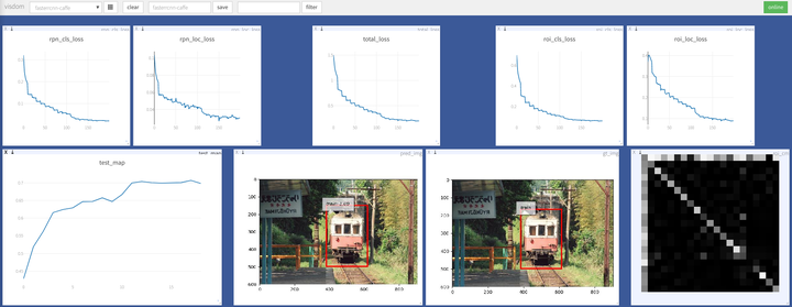
The effect is good enough: higher than the score in the original paper (the paper mAP is 69.9, this project uses the Caffe version VGG16 pretrain parameters to reach 0.70 at the lowest and 0.712 at the highest.)
Fast enough: the fastest on GTX1080Ti GPU can be completed in about 4 hours.
Smaller GPU memory usage: about 3G video memory usage at the lowest.

This article only select part of important factors to illustrate one implementation method of Faster R-CNN, there are plenty of details that are not mentioned, if you want thoroughly understand the implementation and code, please check here to get more information.

References

[1] A Simple and Fast Implementation of Faster R-CNN