Paper - AdderNet: Do We Really Need Multiplications in Deep Learning?

1 Introduction

Origin:

• CVPR 2020 Oral

Author:

• Peking University
• Huawei
• The University of Sydney

Task:

• Energy efficient networks

Existing Methods:

• Network pruning
• Efficient blocks design (e.g. MobileNet, ShuffleNet)
• Knowledge Distillation
• Low-bit Quantization (e.g. Binary Neural Network)

Limitations:

• Containing massive multiplications

Proposed Method:

Today’s convolution operation of convolution neural network (CNN) includes a lot of multiplication. Although there are many lightweight networks (such as MobileNet) proposed, the cost of multiplication is still hard to be ignored. To carry out deep learning application in edge devices, it is necessary to further lower the computation cost and energy consumption, so this paper proposes to use addition operation instead of multiplication operation to perform deep neural networks.

The paper points out that the traditional convolution operation is actually a kind of cross-correlation operation used to measure the similarity between input features and convolution kernels, and this cross-correlation operation introduces many multiplication operations which increase the computation cost and energy consumption, so the paper proposes another way to measure the similarity between input features and convolution kernels, which is $\ell_1$ distance.

2 Method

2.1 Similarity Measurment

Suppose that $F \in \mathbb{R}^{d \times d \times c_{in} \times c_{out}}$, $F$ is the filter of a layer in the middle of the network, the filter size is $d$, the input has $c_{in}$ channels, and the output has $c_{out}$ channels. The input feature is defined as $X \in \mathbb{R}^{H \times W \times c_{in}} $, where $H$ and $W$ correspond to the height and width of the feature. Then the output $Y$ has the following formula:

$$Y(m, n, t)=\sum_{i=0}^{d} \sum_{j=0}^{d} \sum_{k=0}^{c_{i n}} S(X(m+i, n+j, k), F(i, j, k, t)), \tag {1}$$

where $S$ is the similarity function.

2.2 Convolution Kernel

If $S (x, y) = X \times F$, then formula (1) becomes the convolution operation in the traditional convolutional neural network:

$$Y(m, n, t)=\sum_{i=0}^{d} \sum_{j=0}^{d} \sum_{k=0}^{m} X(m+i, n+j, k) \cdot F(i, j, k, t) \tag {2}$$

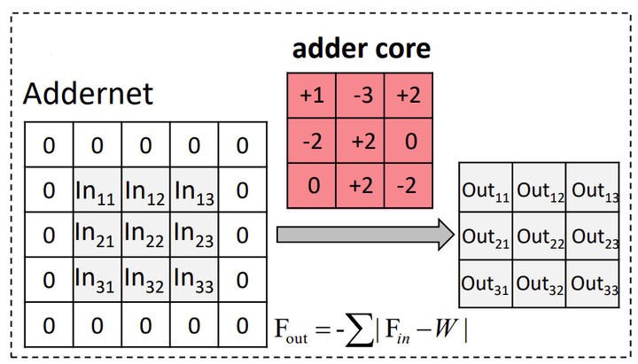
2.3 Addition Kernel

As mentioned above, if $\ell_1$ distance $\left | x \right |_{1} = \left | x_1 \right | + \left | x_2 \right | + \cdots + \left | x_n \right |$ is used instead of cross-correlation operation, then formula (1) becomes:

$$Y(m, n, t)=-\sum_{i=0}^{d} \sum_{j=0}^{d} \sum_{k=0}^{c_{in}}|X(m+i, n+j, k)-F(i, j, k, t)|, \tag {3}$$

here the author mentioned that the results of such operations are all negative, but the output value of the traditional convolutional neural network is positive or negative, therefore, behind the output layer is the Batch Normalization (BN) layer, which makes the output distribution in a reasonable range.

2.4 Optimization

In traditional convolution networks, the back propagation formula of $Y$ about $F$ is as follows:

$$\frac{\partial Y(m, n, t)}{\partial F(i, j, k, t)}=X(m+i, n+j, k) \tag {4}$$

The derivative of $\ell_1$-norm is a piecewise function:

$$\frac{ \partial }{ \partial x } || x ||_1 = \operatorname {sign}(x) \text{, where } \operatorname {sign}(x) = \begin{cases} -1 & x_i<0 \\
+1 & x_i>0 \\
[-1, 1] & x_i=0 \end{cases}$$

In AdderNet, the back propagation formula of $\ell_1$-norm is as follows:

$$\frac{\partial Y(m, n, t)}{\partial F(i, j, k, t)}=\operatorname{sgn}(X(m+i, n+j, k)-F(i, j, k, t)) \tag {5}$$

It is pointed out in the paper that the signSGD of $\ell_1$-norm back propagation cannot decline in the best direction, and it will choose the worse direction sometimes. Therefore, the paper changes the back propagation formula into $\ell_2$-norm back propagation, which is called full precision gradient.

The derivative of $\ell_2$-norm:

$$ \frac{ \partial | | \mathbf{x} | |_2^2 }{ \partial \mathbf{x}} = \frac{ \partial | | \mathbf{x}^T \mathbf{x} | |_2}{ \partial \mathbf{x}} = 2 \mathbf{x} $$

In AdderNet, the back propagation formula of $\ell_2$-norm is as follows:

$$\frac{\partial Y(m, n, t)}{\partial F(i, j, k, t)}=X(m+i, n+j, k)-F(i, j, k, t)$$

Considering the derivative of $Y$ to $X$, according to the chain rule, $\frac{\partial Y}{\partial F_i }$ is only related to $F_i$ itself, while $\frac{\partial Y}{\partial X_i }$ will affects layers before the $i$th layer, which magnified the gradient. This paper use HardTanh function to clip the gradient of $X$ to prevent gradient exploding.

$$\frac{\partial Y(m, n, t)}{\partial X(m+i, n+j, k)}=\operatorname{HT}(F(i, j, k, t)-X(m+i, n+j, k)), \tag {6}$$

$$ where \operatorname{HT}(x) = \begin{cases} x & -1<x<1 \\
-1 & x<-1 \\
1 & x>1 \end{cases} $$

2.5 Adaptive learning rate

In traditional CNN, normally we expect that the output distribution between each layer is similar, so that the weights of the network are more stable. Considering the variance of the output features, we assume that all values in $F$ and $X$ are independent and identically distributed, then the variance in CNN has the following formula:

$$\begin{aligned} \operatorname{Var}\left[Y_{C N N}\right] &=\sum_{i=0}^{d} \sum_{j=0}^{d} \sum_{k=0}^{c_{\text {in }}} \operatorname{Var}[X \times F] \\
&=d^{2} c_{i n} \operatorname{Var}[X] \operatorname{Var}[F] \end{aligned} \tag{7}$$

Similally, the variance in AdderNet has the following formula:

$$\begin{aligned} \operatorname{Var}\left[Y_{\text {AdderNet }}\right] &=\sum_{i=0}^{d} \sum_{j=0}^{d} \sum_{k=0}^{c_{\text {in }}} \operatorname{Var}[|X-F|] \\
&=\left(1-\frac{2}{\pi}\right) d^{2} c_{i n}(\operatorname{Var}[X]+\operatorname{Var}[F]) \end{aligned} \tag{8}$$

The variance of CNN is small because $\operatorname{Var}[F]$ is close to zero, while the variance of AdderNet is much lager than CNN because $\operatorname{Var}[X]$ is large. This paper use BN to normalize the output of a lay to avoid the variance exploding.

In AdderNet, the output of each layer is followed by a BN layer. Although BN layer brings some multiplication operations, the magnitude of these operations can be ignored compared with that of classical convolution network. Given a mini-batch input $B=\{x_1, …, x_m\}$, BN layer can be defined as the following formula:

$$y=\gamma \frac{x-\mu_{B}}{\sigma_{B}}+\beta=\gamma \hat{x}+\beta, \tag{9}$$

where $\gamma$ and $\beta$ are parameters to learn, $\mu$ and $\sigma$ are mean and variance of output.

Then the partial derivation of $x$ after adding BN layer is:

$$\frac{\partial \ell}{\partial x_{i}}=\sum_{j=1}^{m} \frac{\gamma}{m^{2} \sigma_{B}} \left\{ \frac{\partial \ell}{\partial y_{i}}-\frac{\partial \ell}{\partial y_{j}}\left[1+\frac{\left(x_{i}-x_{j}\right)\left(x_{j}-\mu_{B}\right)}{\sigma_{B}}\right] \right\} \tag{10}$$

Since the weight gradient depends on the variance, the weight gradient in the AdderNet with BN layer will be very small. The following table is a comparison:

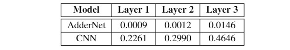
Except for showing a small gradient, the table also shows that some layers may not be of the same magnitude, so it is no longer appropriate to use a global unified learning rate. Therefore, an adaptive learning rate method is used in the paper, making the learning rate different in each layer. Its formula calculation is expressed as:

$$\Delta F_{l}=\gamma \times \alpha_{l} \times \Delta L\left(F_{l}\right), \tag{11}$$

where $\gamma$ is a global learning rate, $\Delta F_{l}$ is the change of the filter in layer $l$, and $\alpha_{l}$ is its corresponding local learning rate.

$$\alpha_{l}=\frac{\eta }{\sqrt{k} \lVert \Delta L\left(F_{i}\right) \lVert_{2}}, \tag{12}$$

where $k$ is the number of elements in $F_l$, $\eta$ is a hyper-parameter to control the learning rate of adder filters.

With such a learning rate adjustment, the learning rate can be automatically adapted to the situation of the current layer in each layer.

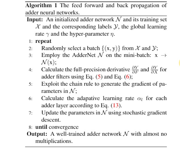
2.6 Training Procedure

The above is all the new ideas and designs proposed in this paper, and the process description of forward and backward propagation of AdderNet is also given in this paper as below.

3 Experiment

See the original paper for the comparison of experimental data and results.

Thinking

When I first read this paper, I thought it was another version of the Binary Neural Network, but after reading it carefully, I found that it was actually a new form of reducing the FLOP. The amount of calculation is a compromise between quantization calculation and full-precision calculation, with a comparable accuracy compared to the traditional CNNs. The storage amount would be larger than quantified CNNs. I think if we can combine other methods (such as quantization, pruning) and other algorithms, there will be more new ideas. It is a direction worth to study.