The Evolution of the Convolutional Neural Networks Architecture
A perspective of understanding CNN
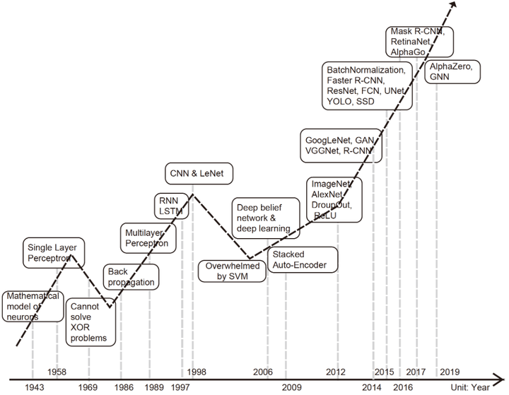
1 The Origin of CNN
The study of artificial intelligence may be traced back to the ancient Greeks Aristotle who proposed Associationism theory in order to explain the operation of the human brain, he probably would not have thought that nowadays, more than 2000 years later, people are using the artificial neural network derived from associationism to build super artificial intelligence.
In the following two thousand years, the associationism theory was supplemented and perfected by many philosophers or psychologists, and finally led to the Hebbian Learning Rules in 1949 by Donald O. Hebb, which became the basis of neural networks. Hebb is also seen as the father of Neural Networks because of this work.
In 1958, Frank Rosenblatt further substantialized HebbianLearning Rule with the introduction of Perceptrons. A perceptron is fundamentally a linear function of input signals, which cannot represent a non-linear decision boundary like XOR. This limitation was highlighted by Minski and Papert in 1969. As a result, very little research was done in this area until about the 1980s.
In 1980, Kunihiko Fukushima proposed Neocogitron which is generally seen as the model that inspires Convolutional Neural Networks on the computation side.
The term Backpropagation and its general use in neural networks was announced by David Rumelhart, Geoffrey Hinton and Ronald J. Williams in 1986, then they elaborated and popularized it, but the technique was independently rediscovered many times, and had many predecessors dating to the 1960s.
In 1989, George Cybenko proved Universal Approximation Theorem, roughly describes that a multi-layer perceptron (MLP) can represent any functions. The universal approximation properties showed a great potential of shallow neural net-works at the price of exponentially many neurons at these layers.
The major milestones before 1986 as shown in the blow table:
| Year | Contributer | Contribution |
|---|---|---|
| 300 BC | Aristotle | introduced Associationism, started the history of human’sattempt to understand brain. |
| 1873 | Alexander Bain | introduced Neural Groupings as the earliest models of neural networks, inspired Hebbian Learning Rule. |
| 1943 | McCulloch & Pitts | introduced MCP Model, which is considered as the ancestor of the Artificial Neural Model. |
| 1949 | Donald Hebb | considered as the father of neural networks, introducedHebbian Learning Rule, which lays the foundation of modern neural networks. |
| 1958 | Frank Rosenblatt | introduced the first perceptron, which highly resembles modern perceptron. |
| 1974 | Paul Werbos | introduced Backpropagation |
| 1980 | Teuvo Kohonen | introduced Self Organizing Map |
| 1980 | Kunihiko Fukushima | introduced Neocogitron, which inspired Convolutional Neural Network |
| 1982 | John Hopfield | introduced Hopfield Network |
| 1985 | Hilton & Sejnowski | introduced Boltzmann Machine |
| 1986 | Paul Smolensky | introduced Harmonium, which is later known as RestrictedBoltzmann Machine |
| 1986 | Michael I. Jordan | defined and introduced Recurrent Neural Network |
2 From NN to CNN - LeNet
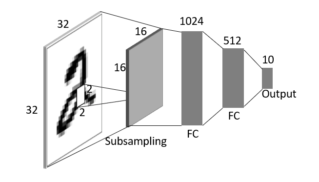
Based on the previous discoveries and research results, a multi-layer perceptron (MLP) neural network model could be used to recognize a figure “2” from an image as below structure.
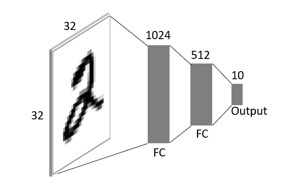
The parameter number are:
32*32*1024+1024*512+512*10+(1024+512+10)=1,579,530
For a 32*32 images, the parameters are way too many. Even more, the above model tends to overfit because each unit of the neural network layer receives the full image.
In 1998, LeNet was invented by Yann LeCun, the first convolutional neural network structure to address the above issues of traditional neural networks. LeNet introduced two most important components: Convolutional Layer and Subsampling Layer.
2.1 Convolutional Layer
A convolutional layer is primarily a layer that performs convolution operation.
Linear operations performed in one domain (time or frequency) have corresponding operations in the other domain, which are sometimes easier to perform and understand. A time domain signal can be transformed to many frequencies in frequency domain as shown in the below figure.
![]()
In 2D space, an image can be transformed to many 2D waves, as shown in the below figure.
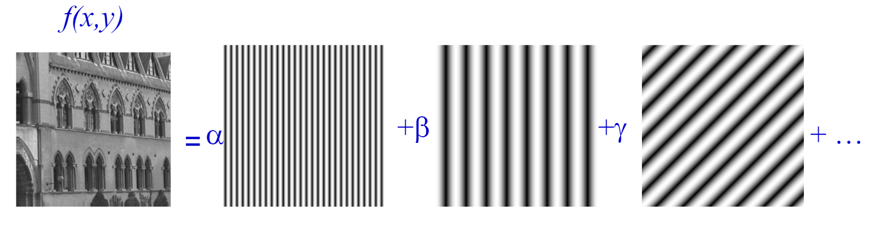
The convolution theorem prooved: space convolution equals frequency multiplication.
$f(x,y)*h(x,y)\Leftrightarrow F(u,v)H(u,v)$
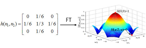
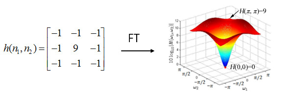
That is to say, the result of the convolution operation is the same as filtering, and a convolution kernel equals a filter. Different convolution kernels applied to the same image will result in differently processed images.
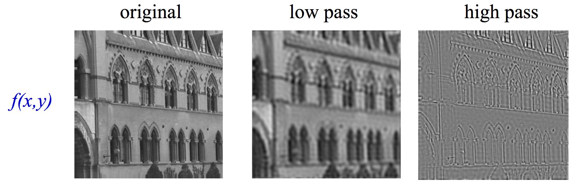
For example, this convolution kernel is a low pass filter, which filters out high frequencies waves (e.g. on the edge of a block) in an image, making an image blurrer.
This convolution kernel is a high pass filter, which filters out low frequencies waves (e.g. inside a block) in an image, making an image sharper.
And the results of different filter:
The convolutional layer introduces another operation after convolution to assist the simulation to be more successful: the non-linearity transform. This non-linearity grants the convolution more power in extracting useful features and allows it to simulate the functions of the visual cortex more closely.
The result after convolution operation (filtering) with a convolution kernal is called the feature map, as the input of next layer.
2.2 Subsampling Layer
The subsampling layer only samples one input out every region looks into, as shown in the below figure. Some different strategies of sampling can be considered, like max-pooling (taking the maximum value of the input), average-pooling (taking the averaged value of input) or even probabilistic pooling (taking a random one).
Sampling turns the input representations into smaller and more manageable embeddings. More importantly, sampling makes the network invariant to small transformations, distortions, and translations in the input image. A small distortion in the input will not change the outcome of pooling since we take the maximum/average value in a local neighbourhood.
2.3 LeNet
With the understanding of the essential role convolution operation plays in vision tasks, we proceed to investigate the previous MLP neural network along the way.
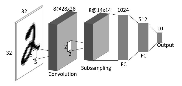
The issues of MLP neural network is huge parameter numbers and overfitting, now adding a subsampling layer is a method to reduce parameters and overfitting, as shown in the below figure.
The parameter number reduce to:
16*16*1024+1024*512+512*10+1024+512+10=793,098
Although reduced nearly half of the parameter number, the input still the original image (half size), and we need to get image features before the full connection layer.
Now try to add convolution layer, as shown in the below figure.
The parameter number go to:
5*5*8+14*14*8*1024+1024*512+512*10+(8+1024+512+10)=2,136,794
The parameter number is higher than the original MLP neural network, and the feature number is small, it is hard to get usefull outcome in the end. To reduce parameters and get more features, we add the second convolution layer as shown in the below figure.
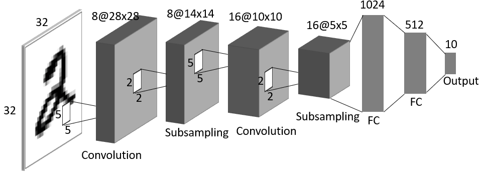
The parameter number reduce to:
5*5*8+5*5*16+5*5*16*1024+1024*512+512*10+(8+16+1024+512+10)=941,178
Now we get a LeNet, the first CNN architecture, which not only reduced the number of parameters but was able to learn features from raw pixels automatically. From LeNet, the three important properties of convolutional neural network are:
- Local receptive fields.
- Shared weights.
- Sub-sampling.
LeNet features can be summarized as:
- Use sequences of 3 layers: convolution, pooling, non-linearity. This may be the key feature of Deep Learning for images since this work.
- Use convolution to extract spatial features.
- Subsample using spatial average of maps.
- Non-linearity in the form of tanh or sigmoids.
- Multi-layer neural network (MLP) as final classifier.
- Sparse connection matrix between layers to avoid large computational cost.
With the success of LeNet, Convolutional Neural Network has been shown with great potential in solving vision tasks. However, a problem was found, that in some cases, the gradient will be vanishingly small, effectively preventing the weight from changing its value. In the worst case, this may completely stop the neural network from further training. In 1991, Sepp Hochreiter’s diploma thesis formally identified the reason for this failure in the “vanishing gradient problem”. Since then, a variety of shallow machine learning models have been proposed, including support vector machine (SVM) invented by Corinna Cortes in 1995, and the research of neural network has been put on hold.
3 The Revival of CNN - AlexNet
While LeNet is the one that starts the era of convolutional neural networks, AlexNet, invented by Alex Krizhevsky (Geoffrey Hinton’s PhD student) in 2012, is the one that starts the era of CNN used for ImageNet classification. AlexNet is the first evidence that CNN can perform well on this historically difficult ImageNet dataset and it performs so well that leads the society into a competition of developing CNNs. The basic layout of the AlexNet architecture as shown in the below figure.
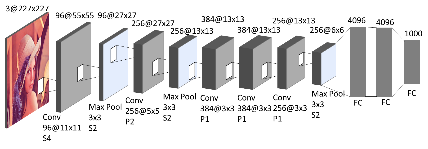
AlexNet scaled the insights of LeNet into a much larger neural network that could be used to learn much more complex objects and object hierarchies. The contribution of this work were:
- Use of rectified linear units (ReLU) as non-linearities to avoid vanishing gradient problem.
- Overlapping max pooling, avoiding the averaging effects of average pooling.
- Local Responce Normalization (LRN) (replaced by Batch Normalization nowadays).
The success of AlexNet is not only due to this unique design of architecture but alsodue to the clever mechanism of training. The training techniques of this work were:
- Data augmentation (random crops/scales etc.) to increase data set.
- Use of dropout technique to selectively ignore single neurons during training, a way to avoid the overfitting of the model.
The success of AlexNet started a small revolution. The convolutional neural network were then the mainstream of Deep Learning.
4 The Rise of CNN - VGG & GoogLeNet
4.1 VGG
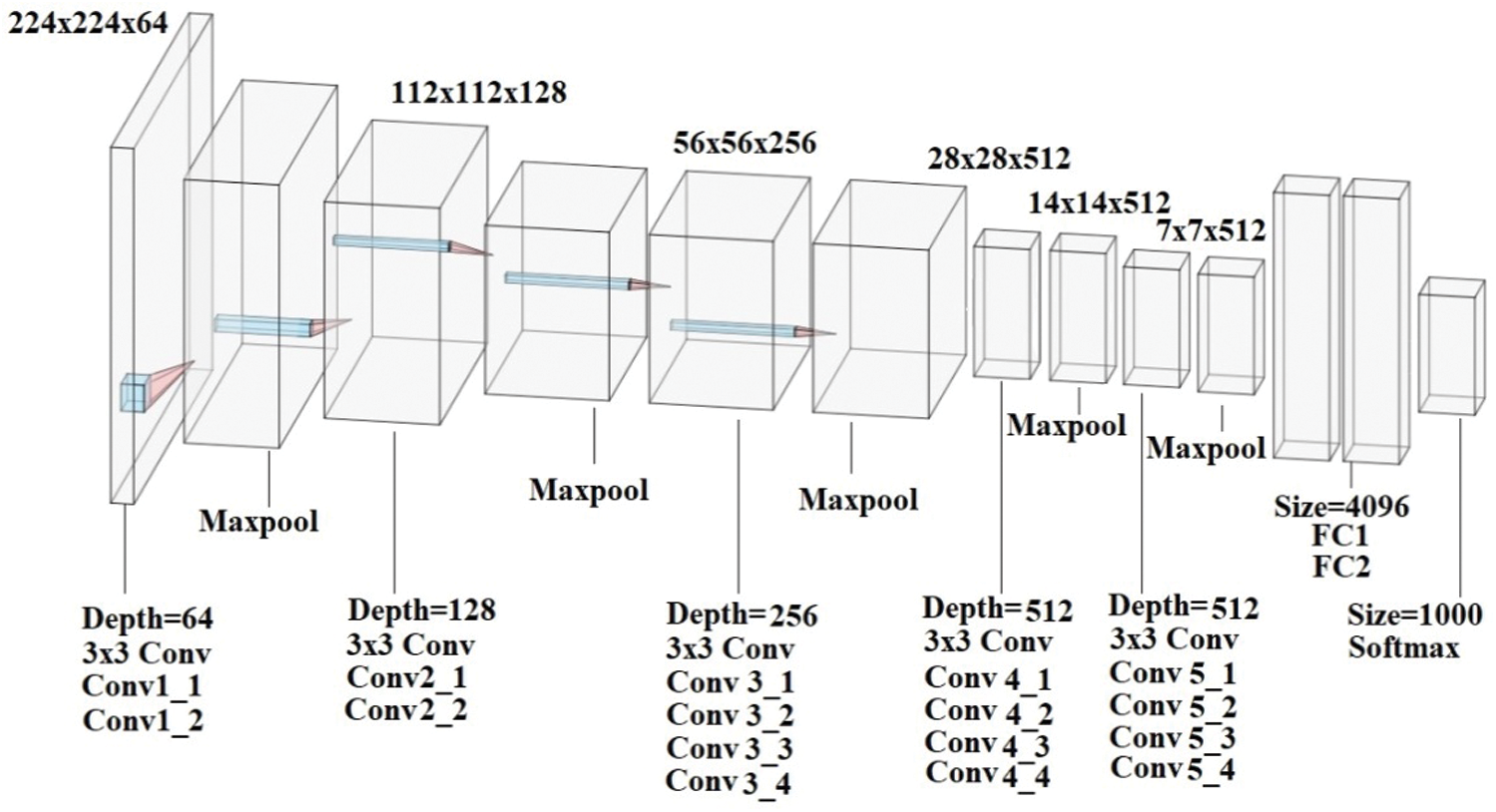
In 2014, Karen Simonyan showed that simplicity is a promising direction with a model named VGG (Visual Geometry Group, the lab Simonyan work for). VGG addresses another very important aspect of convolutional neural networks: depth. Although VGG is deeper (up to 19 layers) than other models around that time, the architecture is extremely simplified: all the layers are 3×3 convolutional layer with a 2×2 pooling layer. The architecture of VGG-19 is as shown in the below figure:
The other configuration of VGG is shown as below table:
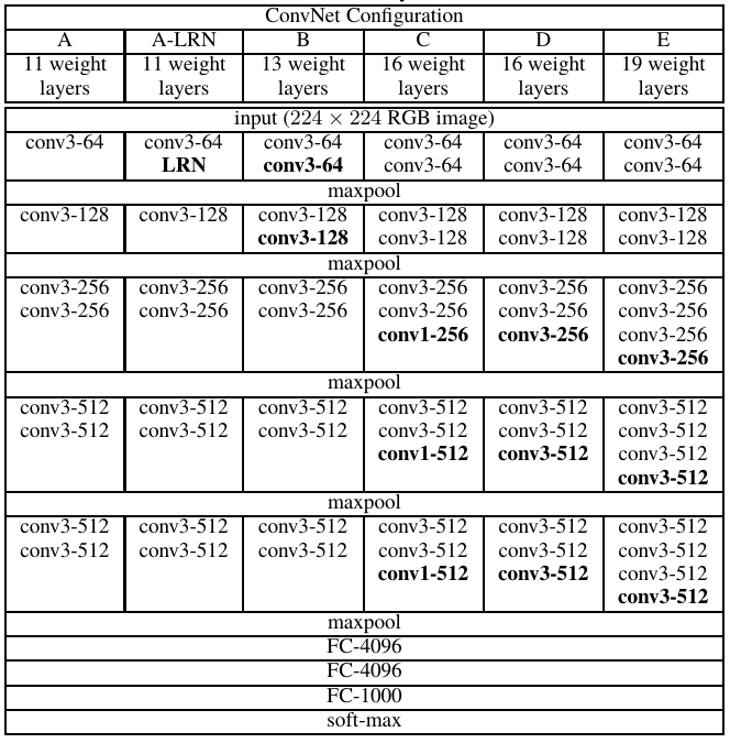
VGG, while based off of AlexNet, has several differences that separates it from other competing models:
- VGG uses very small receptive fields (3x3 with a stride of 1). Because there are now three ReLU units instead of just one, the decision function is more discriminative. There are also fewer parameters.
- VGG incorporates 1x1 convolutional layers to make the decision function more non-linear without changing the receptive fields.
- The small-size convolution filters allows VGG to have a large number of weight layers; and more layers leads to improved performance.
VGG was at 2nd place in the 2014-ILSVRC competition, become famous due to its simplicity, homogenous topology, and increased depth. The main limitation associated with VGG was the use of 138 million parameters, which make it computationally expensive and difficult to deploy it on low resource systems.
4.2 GoogLeNet
GoogLeNet was the winner of the 2014-ILSVRC competition and is also known as Inception-V1. The Google incepton nets are a big family, including:
| Time | Model | Difference | Top-5 Error Rate |
|---|---|---|---|
| Sept. 2014 | Inception V1 | - | 6.67% |
| Feb. 2015 | Inception V2 | 5x5 Conv -> 2*3x3 Conv, Batch Normalization | 4.8% |
| Dec. 2015 | Inception V3 | Factorization into small convolutions, Network In Network In Network | 3.5% |
| Feb. 2016 | Inception V4 | ResNet idea | 3.08% |
The first version entered the field in 2014, and as the name “GoogLeNet” suggests, it was developed by a team at Google. It introduced the new concept of inception block in CNN, whereby it incorporates multi-scale convolutional transformations using split, transform and merge idea. The architecture of the inception block is shown in below figure:

This inception block encapsulates filters of different sizes (1x1, 3x3, and 5x5) to capture spatial information at different scales, including both fine and coarse grain level. This idea helped in addressing a problem related to the learning of diverse types of variations present in the same category of images having different resolutions.
In GoogLeNet, conventional convolutional layers are replaced in small blocks similar to the idea of substituting each layer with Network in Network (NIN) architecture. There are 9 inception modules stacked linearly in total, with 22 layers deep and 27 pooling layers included. The ends of the inception modules are connected to the global average pooling layer to reduce connection’s density. It also introduced the concept of auxiliary learners to speed up the convergence rate. The architecture is shown in the below figure:
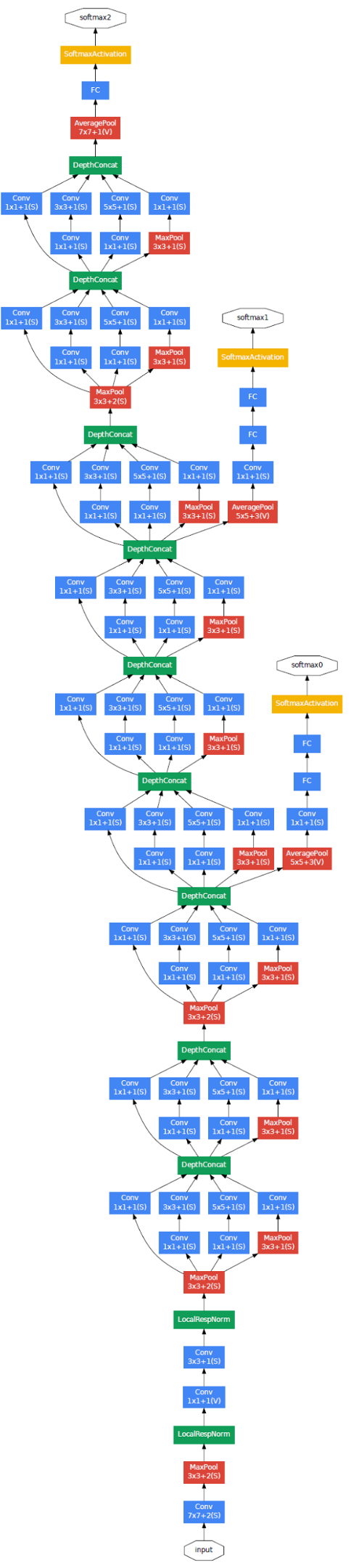
However, the main drawback of the GoogLeNet was its heterogeneous topology that needs to be customized from module to module. Another limitation of GoogLeNet was a representation bottleneck that drastically reduces the feature space in the next layer and thus sometimes may lead to loss of useful information.
5 The blossoming of CNN - ResNet
Following the path VGG introduces, in order to address the problems faced during training of deeper networks, in 2015, Kaiming He invented ResNet (Residual Network) that exploited the idea of bypass pathways used in Highway Networks. The breakthrough ResNet introduces, which allows ResNet to be substantially deeper than previous networks, is called Residual Block, as shown in the blow figure:
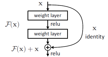
To solve the problem of vanishing/exploding gradients, a skip/shortcut connection is added to add the input x to the output after few weight layers. Hence, the output $H(x)= F(x) + x$. The weight layers actually is to learn a kind of residual mapping: $F(x)=H(x)-x$, which is used to perform reference based optimizationof weights. The distinct feature of ResNet is reference based residual learning framework. ResNet suggested that above residual block are easy to optimize and can gain accuracy forconsiderably increased depth.
The below figure shows the VGG-19, 32 layers plain, and 32 layers ResNet architecture:
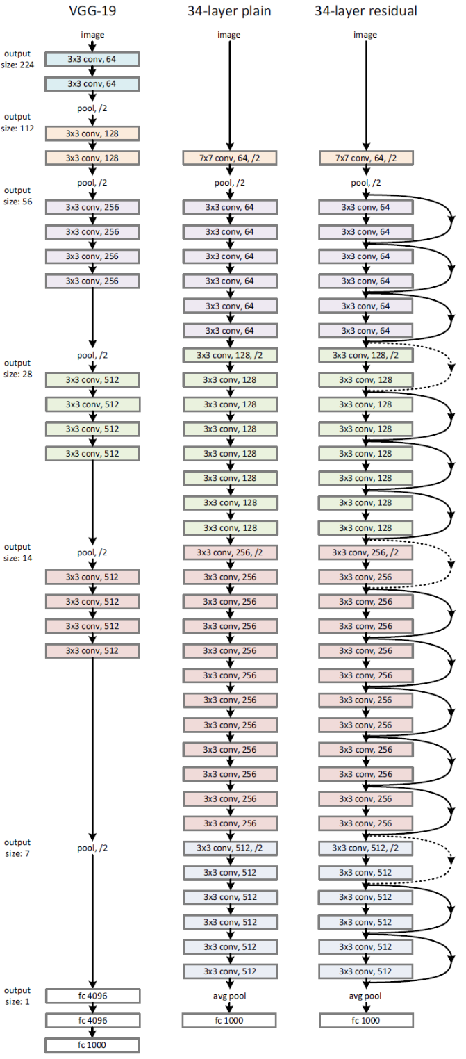
- The VGG-19 (left) is a state-of-the-art approach in ILSVRC 2014.
- 34-layer plain network (middle) is treated as the deeper network of VGG-19, i.e. more convolution layers.
- 34-layer ResNet (right) is the plain one with addition of skip/shortcut connection.
ResNet introduced shortcut connections within layers to enable cross-layer connectivity; however, these connections are data-independent and parameter-free in comparison to the gates of Highway Networks. In Highway Networks, when a gated shortcut is closed, the layers represent non-residual functions. However, in ResNet, residual information is always passed, and identity shortcuts are never closed. Residual links (shortcut connections) speed up the convergence of deep networks, thus giving ResNet the ability to avoid gradient diminishing problems.